Dual-Pivot Binary Search
In 2009, Vladimir Yaroslavski introduced a Dual-Pivot QuickSort algorithm, which is currently the default sorting algorithm for primitive types in Java 8. The idea behind this algorithm is both simple and awesome. Instead of using single pivot element, it uses two pivots that divide an input array into three intervals (against two intervals in original QuickSort). This allowed to decrease the height of recursion tree as well as reduce the number of comparisons. The post describes a similar dual-pivot approach but for a BinarySearch algorithm. Thus, our modified binary search algorithm has prefix Dual-Pivot.
First of all, consider a standard variation of a binary search algorithm.
int binarysearch(int a[], int k, int lo, int hi) {
  if (lo == hi) return -1;

  int p = lo + (hi - lo) / 2;

  if (k < a[p]) {
    return binarysearch(a, k, lo, p);
  } else if (k > a[p]) {
    return binarysearch(a, k, p + 1, hi);
  }

  return p;
}
We’ll use a Master Method in order to understand its time complexity in terms of Big-Oh notation. The idea behind a master method is to express algorithm’s running time in terms of the following recurrent relation.
T(n) = a * T(n/b) + O(n^c)The exact meaning of this relation is following: the running time T(n) of the algorithm on input n is equal to sum of the running times of each recursive call T(n/b) plus some extra job O(n^c) at each level of recursion. Note that a master method only works for Divide and Conquer algorithms.
The binary search algorithm does
- split the input onto two equals intervals:
b = 2 - perform only one recursive call, depending on whether the key is less or greater then the pivot element:
a = 1 - compare the key with the pivot element at each level of recursion, which takes a constant time:
c = 0
Thus, the following recurrent relation describes a standard binary search algorithm, where a = 1 (number of recursive calls), b = 2 (how many pieces we split the data at each level of recursion) and c = 0 (we also do some constant work at each recursion call).
T(n) = T(n/2) + O(1)The relation a == b ^ c or 1 == 2 ^ 0 gives us the first case in a master method, which results in the running time O(n^c * log_b n) or O(log_2 n) in particular.
It’s time to use a dual-pivot element instead of a single-pivot one. This gives us three intervals and a couple of additional comparisons.
int dualPivotBinarysearch(int a[], int k, int lo, int hi) {
  if (lo == hi) return -1;

  int p = lo + (hi - lo) / 3;
  int q = lo + 2 * (hi - lo) / 3;

  if (k < a[p]) {
    return dualPivotBinarysearch(a, k, lo, p);
  } else if (k > a[p] && k < a[q]) {
    return dualPivotBinarysearch(a, k, p + 1, q);
  } else if (k > a[q]) {
    return dualPivotBinarysearch(a, k, q + 1, hi);
  }

  return (k == a[p]) ? p : q;
}
It should be clear now that a recurrent relation for a dual-pivot binary search looks as follows.
T(n) = T(n/3) + O(1)The only difference is a data split factor, which is 3 against 2 in the original relation. Thus, three intervals give us a new time complexity: O(log_3 n). The careful reader may notice, that a logarithm’s base is a constant factor, which is redundant and might be eliminated according to the Big-Oh definition rules. So, both algorithm have the same time bounds - O(log n). And it’s doesn’t really matter what base of log is.
That is a partially true. We usually don’t care about constant factors in asymptotic bounds, since it doesn’t affect the algorithm’s scalability. The only thing we care is whether the algorithm is able to process the bigger (much bigger) input in a reasonable time or not. But, when it comes to a deeper analysis of the particular algorithm implementation, it may be useful keeping in mind the constant factors as well.
The new time complexity gives us a shorter version of a recursive tree: log_3 n against log_2 n. In other words, it gives us a shorter stack trace as well as a smaller memory footprint (due to reduced number of the allocated stack frames). For example, for n = 2 147 483 647 (a maximum length of the array that might be allocated in JVM) we’ll have a 40% shorter recursive tree. Isn’t it awesome? Not really. To be honest, 40% is from difference between 31 and 19 (base 2 against base 3 in a logarithmic function). A logarithm is an awesome function! It takes a number and makes it smaller. I wish all the algorithms have had a logarithm in their asymptotic bounds.
Well, what does it cost to make 31 recursive calls on a modern JVM (and a modern CPU as well)? I bet - nothing. And this might be a strong reason why we didn’t study a dual-pivot binary search algorithm in a university course. Another reason is optimizing compilers (i.e., a HotSpot JIT Compiler) that can easily eliminate a tail-recursion by replacing it with a simple iterative loop. Therefore, all the fictional benefits of using a dual-pivot binary search might be completely lost.
Anyway, there is still an interesting part of a dual-pivot approach that wasn’t discussed yet - a number of comparisons. Using a dual-pivot element introduces a different number of comparisons per recursive call: 4 (against 2 in a classic scheme), which doesn’t sound optimistic, but still should be investigated. And the easiest way to check whether it’s worth to use a dual-pivot scheme or not is to look at graphical representation of both functions: 2 log_2 n and 4 log_3 n.
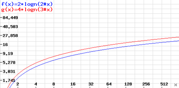
The chart above shows that a dual-pivot scheme uses a bit more comparisons then a single-pivot one on the same input. More precisely, it uses 20% more comparisons then an original algorithm. On the one hand, a dual-pivot approach introduces a shorter recursive tree (less number of recursive calls), but on the other hand - a higher number of comparisons.
Let me do some math in order to find a reasonable answer whether (and when) it’s worth to use a dual-pivot binary search algorithm or not. A couple of new variables should be introduces: p - latency of a recursive (or simple) call, q - latency of a compare operation (i.e., an integer compare). Now we can define the total running time of a binary search algorithm as follows.
t(binary search) = p * log_2 n + 2q * log_2 n It just straightforward: we waste p * log_2 n time doing recursive calls plus 2q * log_2 n doing comparisons. The similar formula might be defined for a dual-pivot binary search algorithm.
t(dual-pivot binary search) = p * log_3 n + 4q * log_3 n And we want to find a relation between q and p for which the following will be true (we’re looking for constraints with which a dual-pivot scheme takes less time).
t(binary search) > t(dual-pivot binary search)

.. or ..

(p * log_2 n) + (2q * log_2 n) > (p * log_3 n) + (4q * log_3 n)
This gives us a strict answer: p > 1.5 q. In other words, it does make sense to use a dual-pivot approach on a platform for which making a function call costs at least as 1.5x of compare operation.
That’s nice to know, but can we find a more concrete answer? Well, it’s not that easy. It really depends on a hardware platform (ISA, micro-architecture) as well as on a software platform (compiler, runtime). Consider we use a compiler without tail-call optimization on a modern Intel’s CPU (like Haswell). An Agner’s optimization manual says that it takes 1 or 2 clock-ticks for both CMP and FUCOMI/FUCOMIP instructions. Needless to say that JMP, SUB and MOV cost almost nothing: ~3-4 clock-ticks in total. Why do we need these three instructions? Well, a usual calling convention does
- perform a jump to a function -
JMP - save the current stack pointer -
MOV - reserve a stack for locals -
SUB
Well, it’s roughly takes 3-4 clock-ticks in order to make a function call on a modern x86 chip. And this almost what we was looking for. We can say that it might be a good idea of using a dual-pivot binary search instead of a classic one. But the benefits we get in this case are such imperceptible that we won’t even see the difference. The only micro-benchmarking will help us find a truth.
The full source code of a JMH-based benchmark is available at GitHub. The results look as follows.
Benchmark                Mode   Samples         Mean   Mean error    Units
d.DPBS.benchmarkBS       avgt         5       81.665        8.000    ns/op
d.DPBS.benchmarkDPBS     avgt         5       69.563        8.410    ns/op
These performance results (70 nanoseconds vs. 80 nanoseconds on a hugest array that I managed to allocate on my MacBook Pro) sums up in a very robust conclusion: a classic binary search algorithm’s fast as hell. Seriously, it’s one of the fastest algorithms around. Just think about we wasted 80 nanoseconds (read it again - nanoseconds) in order to search in 2Gb array. That’s crazy fast and the difference in 10ns (read it again - nanoseconds) is just sort of quantum side-effects. So, if you have a bunch of ordered numbers and you want to perform a search on them - relax and use Arrays.binarySearch() or even write your own implementation for a particular case.
The point is we don’t need a dual-pivot approach, since it gives you almost nothing on a modern platforms. The aim of this post is to find a reasonable answer on a question why there’s still no dual-pivot binary search around. I didn’t want to get a faster version of a original binary search, which surely can be done by rewriting a tail-recursion with iteration (but it’s not even necessary - just think of 31 recursive calls in a wost case). I just wanted to show how use complexity analysis along with math and knowledge about your platform in order to dig into the interesting question and have fun.


